Analyzing Historical Default Rates of Lending Club Notes

In case you're unfamiliar, Lending Club is the world's largest peer-to-peer lending company, offering a platform for borrowers and lenders to work directly with one another, eliminating the need for a financial intermediary like a bank. Removing the middle-man generally allows both borrowers and lenders to benefit from better interest rates than they otherwise would, which makes peer-to-peer lending an attractive proposition. This post will be the first in a series of posts analyzing the probability of default and expected return of Lending Club notes. In this first post, I'll cover some of the background on Lending Club, talk about getting and cleaning the loan data, and perform some exploratory analysis on the available variables and outcomes. In subsequent posts, I'll work on developing a predictive model for determining the loan default probabilities. Before investing, it is always important to fully understand the risks, and this post does not constitute investment advice in either Lending Club or in Lending Club notes.

Background and Gathering Data

Lending Club makes all past borrower data freely available on their website for review, and I will be referencing the 2012-2013 data throughout this post.

To download the 2012-2013 data from Lending Club:

# Download and extract data from Lending Club
if (!file.exists("LoanStats3b.csv")) {
    fileUrl <- "https://resources.lendingclub.com/LoanStats3b.csv.zip"
    download.file(fileUrl, destfile = "LoanStats3b.csv.zip", method="curl")
    dateDownloaded <- date()
    unzip("LoanStats3b.csv.zip")
}

# Read in Lending Club Data
if (!exists("full_dataset")) {
  full_dataset <- read.csv(file="LoanStats3b.csv", header=TRUE, skip = 1)
}

For each loan in the file, Lending Club provides an indication of the current loan status. Because many of the loan statuses represent similar outcomes, I've mapped them from Lending Club's 7 down to only 2, simplifying the problem of classifying loan outcomes without much loss of information useful for investment decisions. My two outcomes "Performing" and "NonPerforming" seek to separate those loans likely to pay in full from those likely to default. Below I include a table summarizing the mappings:

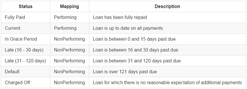
Now that we've loaded the data, let's extract the fields we need and do some cleaning. We can eliminate any fields that would not have been known at the time of issuance, as we'll be trying to make decisions on loan investments using available pre-issuance data. We can also eliminate a few indicative data fields that are repetitive or too granular to be analyzed, and make some formatting changes to get the data ready for analysis. Finally, we'll map the loan statuses to the binary "Performing" and "NonPerforming" classifiers as discussed above.

# Select variables to keep and subset the data
variables <- c("id", "loan_amnt", "term", "int_rate", "installment", "grade", 
               "sub_grade", "emp_length", "home_ownership", "annual_inc", 
               "is_inc_v", "loan_status", "purpose", "addr_state", "dti", 
               "delinq_2yrs", "earliest_cr_line", "inq_last_6mths", 
               "mths_since_last_delinq", "mths_since_last_record", "open_acc", 
               "pub_rec", "revol_bal", "revol_util", "total_acc", 
               "initial_list_status", "collections_12_mths_ex_med", 
               "mths_since_last_major_derog")
train <- full_dataset[variables]


# Reduce loan status to binary "Performing" and "NonPerforming" Measures:
train$new_status <- factor(ifelse(train$loan_status %in% c("Current", "Fully Paid"), 
                                  "Performing", "NonPerforming"))

# Convert a subset of the numeric variables to factors
train$delinq_2yrs <- factor(train$delinq_2yrs)
train$inq_last_6mths <- factor(train$inq_last_6mths)
train$open_acc <- factor(train$open_acc)
train$pub_rec <- factor(train$pub_rec)
train$total_acc <- factor(train$total_acc)

# Convert interest rate numbers to numeric (strip percent signs)
train$int_rate <- as.numeric(sub("%", "", train$int_rate))
train$revol_util <- as.numeric(sub("%", "", train$revol_util))

Analyzing Predictive Power of Variables

Lending Club Grades and Subgrades

All types of borrowers are using peer-to-peer lending for a variety of purposes. This raises the question of how to determine appropriate interest rates given the varying levels of risk across borrowers. Luckily for us, Lending Club handles this for us. They use an algorithm to determine a borrower's level of risk, and then set the interest rates according to the level of risk. Specifically, Lending Club maps borrowers to a series of grades [A-F] and subgrades [A-F][1-5] based on their risk profile. Loans in each subgrade are then given appropriate interest rates. The specific rates will change over time according to market conditions, but generally they will fall within a tight range for each subgrade.

Let's take a look at the proportions of performing and non-performing loans by Lending Club's provided grades:

by_grade <- table(train$new_status, train$grade, exclude="")
prop_grade <- prop.table(by_grade,2)
barplot(prop_grade, main = "Loan Performance by Grade", xlab = "Grade", 
        col=c("darkblue","red"), legend = rownames(prop_grade))

by_subgrade <- table(train$new_status, train$sub_grade, exclude="")
prop_subgrade <- prop.table(by_subgrade,2)
barplot(prop_subgrade, main = "Loan Performance by Sub Grade", xlab = "SubGrade",
        col=c("darkblue","red"),legend = rownames(prop_subgrade))

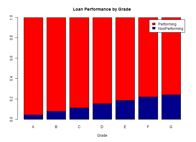
We can see from the chart below that rates of default steadily increase as the loan grades worsen from A to G, as expected.

We see a similar pattern for the subgrades, although the trend begins to weaken across the G1-G5 subgrades. On further investigation, I found that there are only a few hundred data points for each of these subgrades, in contrast to thousands of data points for the A-F subgrades, and these differences are not large enough to be significant.

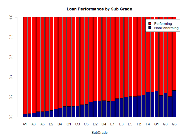
In general, it looks like the Lending Club grading system does a pretty great job of predicting ultimate loan performance, but let's check out some of the other available data to see what other trends we might be able to find in the data.

Home Ownership

The Lending Club data has 3 main classifications for home ownership: mortgage (outstanding mortgage payment), own (home is owned outright), and rent. I would expect those with mortgages to default less frequently than those who rent, both because there are credit requirements to get a mortgage and because those with mortgages might in general tend to be more established. Let's see whether this is actually the case:

ownership_status <- table(train$new_status,train$home_ownership,
                     exclude=c("OTHER","NONE",""))

prop_ownership <- round(prop.table(ownership_status, 2) * 100, 2)

So those with mortgages default the least, followed by those who own their homes outright and finally those who rent. The differences here are much smaller than when comparing different grades, but they are still notable. Let's verify whether these are statistically significant:

# Calculate the counts of mortgage, owners, and renters:
count_m <- sum(train$home_ownership == "MORTGAGE")
count_o <- sum(train$home_ownership == "OWN")
count_r <- sum(train$home_ownership == "RENT")

# Calculate the counts of default for mortgages, owners, and renters:
dflt_m <- sum(train$home_ownership == "MORTGAGE" & train$new_status == "NonPerforming")
dflt_o <- sum(train$home_ownership == "OWN" & train$new_status == "NonPerforming")
dflt_r <- sum(train$home_ownership == "RENT" & train$new_status == "NonPerforming")

# 1-sided proportion test for mortgage vs owners
prop.test(c(dflt_m,dflt_o), c(count_m,count_o), alternative = "less")

# 1-sided proportion test for owners vs renters
prop.test(c(dflt_o,dflt_r), c(count_o,count_r), alternative = "less")

The p-value of the first test was 6.377*10^-12 and the p-value for the second test was 3.787*10^-8, indicating that the differences in both of these proportions are very statistically significant. Although the differences in the default probabilities are somewhat small, on the order of 1.5%, the number of data points is in the high tens of thousands, which contributes to the significance. Given this result, we can generally conclude that similar differences in default probabilities for other factors should also be significant, so long as a similar quantity of data points is available.

Note: for the remaining analysis, the code for each variable becomes a bit repetitive, so in the interest of minimizing the length of this post I will present only the results. If you are interested to see the actual code, you will find it in the appendix at the bottom of this post. You can also read the complete code on Github.

Debt to Income Ratio

Debt to income ratio indicates the ratio between a borrowers monthly debt payment and monthly income. This was originally formatted as a continuous numerical variable, but I bucketed it into 5% increments to better visualize the effect on loan performance. As we might expect, there is a steady increase in the percentage of non-performing loans as DTI increases, reflecting the constraints that increased debt put onto borrower ability to repay:

Revolving Utilization Percent

Revolving utilization percent is the portion of a borrower's revolving credit limit (i.e. credit card limit) that they actually are using at any given point. For example, if a borrower's total credit limit is $15,000 and their outstanding balance is $1,500 their utilization rate would be 10%. We can see below that the percentage of non-performing loans steadily increases with utilization rate. Borrowers with high utilization rates are more likely to have high fixed credit card payments which might affect their ability to repay their loans. Also, a high utilization rate often reflects a lack of other financing options, with borrowers turning to peer-to-peer lending as a last resort. This is in contrast to those borrowers with low utilization rates, who may be using peer-to-peer lending opportunistically to pursue lower interest payments.

Loan Purpose

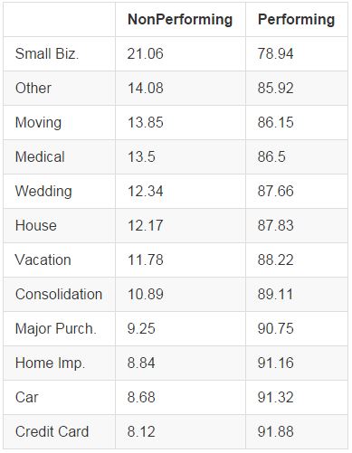
Loan purpose refers to the borrower's stated reason for taking out the loan. We see below that credit card and debt consolidation tend to have better performance, along with home improvement, cars, and other major purchases. Luxury spending on vacations and weddings and unexpected medical and moving expenses generally have worse performance. Small business loans perform very poorly, perhaps reflecting the fact that those borrowers unable to get bank financing for their small business may have poor credit or business plans that aren't fully developed.

Inquiries in the Past 6 Months

Number of inquiries refers to the number of times a borrower's credit report is accessed by financial institutions, which generally happens when the borrower is seeking a loan or credit line. More inquiries leads to higher rates of nonperformance, perhaps indicating that increased borrower desperation to access credit might highlight poor financial health. Interestingly, we see an increase in loan performance in the 4+ inquiries bucket. These high levels of inquiries may reflect financially savvy borrowers shopping around for mortgage loans or credit cards.

Number of Total Accounts

A larger number of total accounts indicates a longer credit history and a high level of trust between the borrower and financial institutions, both of which point to financial health and lower rates of default. We see steady increases in the rates of performing loans as the number of accounts increases from 7 to around 20, but diminishing effects after that.

Annual Income

As we might expect, the higher a borrower's annual income the more likely they are to be able to repay their loans. Below I've broken the income data into quintiles, and we can see that those in the top 20% of annual incomes ($95000 +) are approximately 6% more likely to be performing borrowers than those in the bottom 20% (less than $42000).

Loan Amount

As the amount borrowed increases, we see increasing rates of nonperforming loans. The difference between the first two buckets is only around 1% (and the intra-bucket differences are very small), but we see a larger decrease in loan quality in the $30,000 - $35,000 bucket. Noting that the Lending Club maximum loan is $35,000, this may indicate particularly desperate borrowers who are maximizing their possible borrowing.

Employment Length

We'd expect those who have been employed longer to be more stable, and thus less likely to default. Looking into the data, 3 key groups emerged: the unemployed, those employed less than 10 years, and those employed for 10+ years:

Delinquencies in the Past 2 Years

The number of delinquencies in the past 2 years indicates the number of times a borrower has been behind on payments. I combined all values 3 or larger into a single bucket for analysis, as this was a long right-tailed distribution. Interestingly, those with a single delinquency seem to perform more often than those with none. In general however, the differences between 0, 1, and 2 delinquencies are relatively small, while those with greater than 3 show a significant decrease in performance.

Number of Open Accounts

Unlike the number of total accounts above, which we saw to be quite significant, the number of open accounts variable was not a particularly strong indicator:

Verified Income Status

Lending Club categorizes income verification into three statuses: not verified, source verified, and verified. Verified income means that Lending Club independently verified both the source and size of reported income, source verified means that they verified only the source of the income, and not verified means there was no independent verification of the reported values. Interestingly, we see that as income verification increases, the loan performance actually worsens. During the mortgage crisis, non-verified "no-doc" loans were among the worst performing, so the reversal here is interesting. This likely reflects the fact that Lending Club only verifies those borrowers who seem to be of worse credit quality, so there may be confounding variables present here.

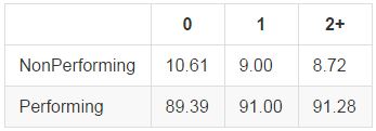
Number of Public Records

Public records generally refer to bankruptcies, so we would expect those with more public records to show worse performance. Actually, performance increases as we move from 0 to 1 to 2 public records. This possibly indicates stricter lending standards from Lending Club on those borrowers with public records:

Variables that were not significant:

• Months since last delinquency
• Months since last major derogatory note
• Collections previous 12 months (too few data points on which to make any conclusions or form predictions)

Summary

• Lending club grade and subgrade variables provide the most predictive power for determining expected loan performance.
• A large number of the other variables also provide strong indications of expected performance. Among the most telling are debt-to-income ratio, credit utilization rate, home ownership status, loan purpose, annual income, inquiries in the past 6 months, and number of total accounts.
• Verified income status and number of public records show results opposite from what we would expect. This is likely due to increased standards on borrowers with poorer credit history, so all else equal we see outperformance in these loans.

We've gotten a good understanding of the available borrower data, and we've seen which variables give the best indiciations of future loan performance. In the next post, We'll work on developing a predictive model for projecting the probability of default for newly issued loans.

Appendix

Below I've included the code used to generate the numbers in the tables above. You can also find the complete code available on Github

### Explore the relationships between default rates and factor levels
### I take a few different approaches, but the key idea is the same


# Home Ownership (exclude status "OTHER" and "NONE" because of few data points)
home_ownership <- table(train$new_status,train$home_ownership,
                     exclude=c("OTHER","NONE",""))
prop_home_ownership <- round(prop.table(home_ownership, 2) * 100, 2)

# Test for significance of the difference in proportions for home ownership factors
# Calculate the counts of mortgage, owners, and renters:
count_m <- sum(train$home_ownership == "MORTGAGE")
count_o <- sum(train$home_ownership == "OWN")
count_r <- sum(train$home_ownership == "RENT")

# Calculate the counts of default for mortgages, owners, and renters:
dflt_m <- sum(train$home_ownership == "MORTGAGE" & train$new_status == "NonPerforming")
dflt_o <- sum(train$home_ownership == "OWN" & train$new_status == "NonPerforming")
dflt_r <- sum(train$home_ownership == "RENT" & train$new_status == "NonPerforming")

# 1-sided proportion test for mortgage vs owners
prop.test(c(dflt_m,dflt_o), c(count_m,count_o), alternative = "less")
# 1-sided proportion test for owners vs renters
prop.test(c(dflt_o,dflt_r), c(count_o,count_r), alternative = "less")


# Debt to Income Ratio (break into factors at 5% levels)
train$new_dti <- cut(train$dti, breaks = c(0, 5, 10, 15, 20, 25, 30, 35))
dti <- table(train$new_status, train$new_dti)
prop_dti <- round(prop.table(dti, 2) * 100, 2)


# Revolving Utilization (break into 0 - 20, then factors of 10, then 80+)
train$new_revol_util <- cut(train$revol_util, breaks = c(0, 20, 30, 40, 50, 60, 70, 80, 141))
revol_util <- table(train$new_status, train$new_revol_util)
prop_revol_util <- round(prop.table(revol_util, 2) * 100, 2)


# Loan Purpose (exclude renewable energy because so few data points)
purpose <- table(train$new_status,train$purpose, exclude = c("renewable_energy",""))
prop_purpose <- round(prop.table(purpose, 2) * 100, 2)


# Inquiries in the last 6 months (combine factor levels for any > 4)
levels(train$inq_last_6mths) <- c("0", "1", "2", "3", rep("4+", 5))
inq_last_6mths <- table(train$new_status, train$inq_last_6mths)
prop_inq_last_6mths <- round(prop.table(inq_last_6mths, 2) * 100, 2)


# Number of total accounts (combine factor levels into groups of 5, then 23+)
levels(train$total_acc) <- c(rep("<= 7", 5), rep("8 - 12", 5), 
                             rep("13 - 17", 5), rep("18 - 22", 5), 
                             rep("23+", 68))
total_acc <- table(train$new_status, train$total_acc)
prop_total_acc <- round(prop.table(total_acc, 2) * 100, 2)


# Annual Income (factor into quantiles of 20%)
train$new_annual_inc <- cut(train$annual_inc,
                            quantile(train$annual_inc, na.rm = TRUE,
                                     probs = c(0, 0.2, 0.4, 0.6, 0.8, 1)))
annual_inc <- table(train$new_status, train$new_annual_inc)
prop_annual_inc <- round(prop.table(annual_inc, 2) * 100, 2)


# Loan Amount (break into < 15k, 15k - 30k, 30k - 35k)
train$new_loan_amnt <- cut(train$loan_amnt,c(0, 15000, 30000, 35000))
loan_amnt <- table(train$new_status, train$new_loan_amnt)
prop_loan_amnt <- round(prop.table(loan_amnt, 2) * 100, 2)


# Employment Length (combine factor levels for better comparison)
levels(train$emp_length) <- c("None", "< 10 years", "< 10 years", "10+ years",
                              rep("< 10 years", 8), "None")
emp_length <- table(train$new_status, train$emp_length)
prop_emp_length <- round(prop.table(emp_length, 2) * 100, 2)


# Delinquencies in the past 2 Years (combine factors levels for any > 3)
levels(train$delinq_2yrs) <- c("0", "1", "2", rep("3+", 17))
delinq_2yrs <- table(train$new_status, train$delinq_2yrs)
prop_delinq_2yrs <- round(prop.table(delinq_2yrs, 2) * 100, 2)


# Number of Open Accounts (combine factor levels into groups of 5)
levels(train$open_acc) <- c(rep("<= 5", 6), rep("6 - 10", 5), 
                            rep("11 - 15", 5), rep("16+", 38))
open_acc <- table(train$new_status, train$open_acc)
prop_open_acc <- round(prop.table(open_acc, 2) * 100, 2)


# Verified income status
is_inc_v <- table(train$new_status, train$is_inc_v, exclude = "")
prop_is_inc_v <- round(prop.table(is_inc_v, 2) * 100, 2)


# Number of Public Records (break factor levels into 0, 1, 2+)
levels(train$pub_rec) <- c("0", "1", rep("2+", 12))
pub_rec <- table(train$new_status, train$pub_rec)
prop_pub_rec <- round(prop.table(pub_rec, 2) * 100, 2)


# Months Since Last Record (compare blank vs. non-blank)
na_last_record <- sum(is.na(train$mths_since_last_record))
not_na_last_record <- sum(!is.na(train$mths_since_last_record))
na_last_rec_dflt <- sum(is.na(train$mths_since_last_record) & train$new_status == "NonPerforming")
not_na_last_rec_dflt <- sum(!is.na(train$mths_since_last_record) & train$new_status == "NonPerforming")

not_na_last_rec_pct_dflt <- not_na_last_rec_dflt / not_na_last_record
na_last_rec_pct_dflt <- na_last_rec_dflt/na_last_record


# Months since last delinquency (break factor levels in increments of 10)
train$mths_since_last_delinq <- cut(train$mths_since_last_delinq, 
                                   breaks = c(0, 10, 20, 30, 40, 50, 60, 156))
mths_since_last_delinq <- table(train$new_status, train$mths_since_last_delinq)
prop_mths_since_last_delinq <- round(prop.table(mths_since_last_delinq, 2) * 100, 2)


# Collections last 12 months
collections <- table(train$new_status, train$collections_12_mths_ex_med)
prop_collections <- round(prop.table(collections, 2) * 100, 2)